We are all familiar with the story of David and Goliath, a shepherd who has defeated a mighty warrior, and the allegory of the underdog beating the giant. Is this story applicable to “People Analytics”?
In our fictional battle today, the giant would be R, the super-power open-source programming language. The underdog would be DMWay, the “new kid in town”: An Israeli start-up that develops an AI approach to predictive analytics, and claims to enable faster and better predictive models. Will their combat end as the old myth? Which of the two rivals enables us to build better predictive models? What can we learn from their contest about “People Analytics” practices? Let’s begin the fight in the arena of predicting employee attrition.
(To explore the R code used in this article, check my GitHub).
Table of Contents
- Employee attrition data
- The cost of employee attrition
- How to predict attrition?
- Logistic regression: R vs DMWay
- The next step: Deployment
- And the winner is…?
- Infographics
Employee attrition data
The reason why our first round in this fictional battle is chosen to be employee attrition lies in the sad reality of HR open data. In a previous post, I mentioned how great it would be to practice analysis and coding based on HR open data. Indeed, it was really encouraging for me to stumble into an employee attrition case, and yet, it was the only open data I found. Nonetheless, employee attrition is a severe problem for many organizations, as I specify below, so both competing technologies, R and DMWay, may offer valuable analysis.
The dataset for the following comparison between R and DMWay was downloaded from Kaggle, a platform for data science competitions, where data scientists can help organizations to solve problems by accurate algorithms based on real data. But not all datasets on Kaggle are real. Datasets published by users on the open data platform are different from those associated with competitions. Some users publish simulated data just for fun or for practice. Unfortunately, that is the case with this employee attrition data.
The dataset titled Human Resources Analytics includes some variables from the realm of HR: numeric variables, e.g., employee satisfaction, employee evaluation, average monthly hours, tenure, and amount of projects, and categorical variables, e.g., work accidents, promotion in last 5 years, department, and salary level. All of these variables may predict the outcome of employee attrition: voluntarily leaving the company. The case study addresses a specific question: “Why are our best and most experienced employees leaving prematurely?” Answering this question would enable this fiction organization to take some actions in order to eliminate or decrease the undesirable outcomes.
At first sight, or rather, by exploring the variables, it seems that the dataset was well simulated as if it was derived from a real HR database. The codebook available is not detailed enough for deeply understanding the meaning of all variables’ units. However, you may assume that some variables would have been re-coded or calculated (e.g., salary level), and others were excluded (e.g., demographics), for the sake of confidentiality. In addition, the data is well structured and clean, in a way you would not expect in case of real data extracted from the HR information system. Nevertheless, let’s continue, assuming that this tidy data is real and complete.
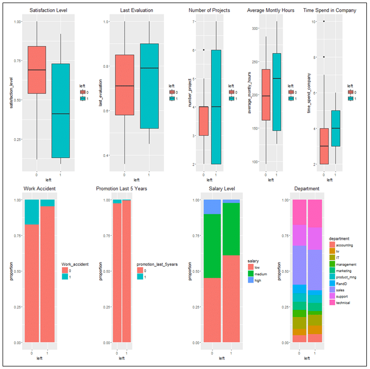
Data exploration reveals that employees who left the company are actually better, in comparison to those who stayed. As shown in Figure 1, although less satisfied and rewarded, employees who left are better evaluated, are involved in more projects, work more, have longer tenure, and are less involved in accidents. These results imply the enormous costs of employee attrition.
Figure 1: Employees who left the company in comparison to those who stayed
(Employees who left – “1”, Employee who stayed – “0”)
The cost of employee attrition
Employee attrition is a huge issue for organizations in every industry. An organization can’t completely avoid employee turnover and attrition, but the rate of employees walking out the door may determine the organization’s doom.
Employees who leave take a significant value with them: professional knowledge, specific practices and know-how, relations within the organization and outside (with clients, suppliers, business partners, etc.), and more. But the damage does not end with this. There are enormous costs, sometimes up to the sum of few salaries per employee, which are tied to recruitment, onboarding, training, and ramping up of a new employee. Furthermore, an organization must take into account some alternative costs, namely the value of transactions that could have been made by a senior employee who actually left.
Indeed, understanding the attrition cost is recommended as the first step in any predictive analytics project. Modeling cost is an effective way to determine ROI (return on investment) of a predictive analytics project that addresses the issue of employee attrition. No wonder why analysts, in companies like Walmart, take the effort to demonstrate to management that reducing even a 1% attrition rate sometimes saves millions of dollars. Although modeling attrition costs is inapplicable in our simulated data, it is important to keep in mind that in a real project it would be a good practice to start with that. Furthermore, a decrease in attrition rate in this imaginary organization (31%) may not only save the recruitment and onboarding cost but probably reduce the alternative costs, since, in this example, employees who leave are considered to be the better ones.
How to predict attrition
There are many modeling techniques that can be used to explain or predict attrition. However, in this article, I have chosen to cover the logistic regression. There are two reasons for my choice: First, the logistic regression is easier to interpret. It may not be the most accurate model, but it offers a pretty good solution without much effort. I believe that in the HR realm, the reasonable way to progress with predictive analytics is generally through good variable selection, that can be easily explained, and not by showing off with excessive models. Second, the objective of this article is not only to demonstrate the implementation of predictive analytics for employee attrition but rather to compare two technologies: R vs DMWay. Since the innovative solution of DMWay relies on regression models, it is more practical to compare the workflow and results of these two technologies by the same modeling.
When analyzing attrition, the goal is essentially to explain or predict a binary or logical variable (voluntary leaving the company) by various other available variables (in this simulation, all or some of the following: employee satisfaction, employee evaluation, average monthly hours, tenure, number of projects, work accidents, promotion in last 5 years, department, and salary level). There are plenty of resources on how Logistic Regression works, but in a nutshell, logistic regression is suited for examining the relationship between a categorical response variable and one or more categorical or continuous predictor variables. It creates an equation that in effect predicts the likelihood of a two-category outcome using the selected predictors. Each of the predictors is associated with a significance mark (p-value) that indicates if the predictor is useful or not.
The implementation of logistic regression, both in R and DMWay, follows the same recipe: data partition into training and testing sets, using logistic regression to model attrition as a function of other predictors in the training dataset, evaluate the model by predicting attrition in the testing dataset, and analyzing how good the model is in terms of prediction accuracy and predictors’ importance. I followed these exact steps in the two technologies but had a totally different user experience, and even different results.
Logistic regression: R vs DMWay
The R output of the logistic regression model is presented in figure 2. This is the fourth model I created, in an effort to generate the most accurate model, as specified below. In this model, all variables were included, except the department variable. Furthermore, the data were subset to include only highly evaluated, senior employees, who work full time. This is appropriate for the simulation objective: “Why are our best and most experienced employees leaving prematurely?” For the purpose of simplicity, and due to the lack of demographics, e.g., gender, the model does not include interactions of variables.
Figure 2: R output of the logistic regression model
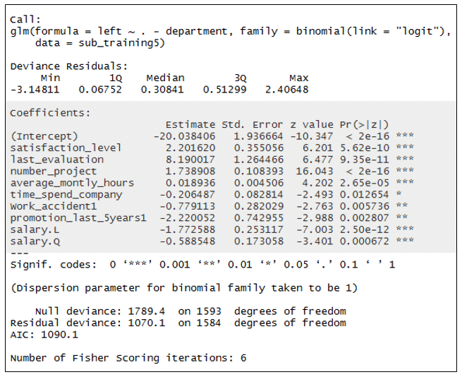
A quick orientation in the model results: The variable names are listed on the far left under “Coefficients”. In the case of categorical variables, the first value (e.g., “0” in work accident) is considered as a baseline, and other values are included in a separate line, indicating their impact relative to the variable baseline. The significance values are provided on the far right under Pr>(|z|). In our case all variables’ estimates have significant value (equal to or lower than 0.05), i.e., they are unlikely to be obtained by pure chance.
Not surprisingly, the intention to leave the company has a negative relation with many variables. Specifically, being promoted, having a medium or high salary, seniority accumulation, and also work accident, decrease the intention to leave. On the other hand, excessive working hours, the number of projects, the last evaluation, and also satisfaction level, have a positive correlation with the intention to leave.
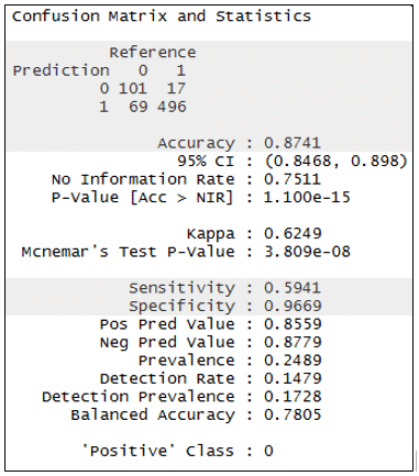
The model output seems straightforward. It implies what the fiction organization should do in order to keep its best employee. But is it accurate? To figure this out, it’s time to use the model to predict the outcomes in the test dataset. The results enable us to build a “confusion matrix”, in which predicted results are compared to observed results. As shown in Figure 3, which is again R output, the prediction is not perfect. The model “was right” in about 87% of the case. The model “specificity”, i.e., its ability to correctly identify those who left is about 97%, whereas the model “sensitivity”, i.e., its ability to correctly identify those who stayed is about 59%.
Figure 3: R output for evaluation of logistic regression model
Another way to evaluate this logistic regression model, and to compare it later to the model made by DMWay, is the AUC, which stands for Area Under the ROC Curve. To make a very very long story short, the “ROC curve” helps to figure out the trade-off between true positive rate (e.g., employees predicted and actually stayed in the company) and false positive rate (e.g., employees predicted to stay but actually left the company), in different cutoff points of prediction, ranged from 0 to 1. In our model, the cutoff point was 0.5, meaning that predicted results equal or above it was considered as “left”. But we could choose other cutoff points and maybe gain better results. With different cutoff values, we move along a curve, where at each point we have different true positive and false-positive rates. Higher and steeper ROC curves are desired and are indicated by a higher area under it (AUC). The perfect theoretical model would have an AUC of 1, and a completely non-predictive model would have an AUC of 0.5. What about our model? It is actually pretty good, but not excellent. It has an AUC of 0.78.
Here we end our session in R and move forward to DMWay. How different the UX is in this software? Will we end up the process with a similar model and predictions? It is worth to mention that each step that was done so far in R was involved with coding because that’s what R is all about. In DMWay, however, the whole process is latent, and the user needs only to make some simple selections in only 4 menus. To illustrate how easy it is to start working with DMWay, you can simply watch this 7min video in which a model is generated and deployed. However, in order to understand and evaluate it, you must already be familiar with the process of predictive analytics, though our R session already gave you the general idea.
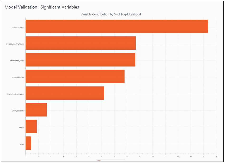
I used the same simulated data, clicked buttons to run a model, since not even a single line of code is needed in DMWay, and then… Wow! The results were stunning. Take a look at the model ROC curve in figure 4, with AUC as perfect as 0.96! But what is the model behind this impressive chart? Exploring the model, as shown in figure5 reveals interesting points: First, the excluded variable here is the promotion, while in the R session I excluded the department. Second, some other variables that do include in the model appear in a piecewise mode, i.e., each of their values range has a different coefficient, hence, different influence on the predictive outcome. That is the reason why there is no need to take a subset of excellent employees to extract a good model, as I did in the R session. I must admit, though, that at first sight, the variety of lines in the model output makes it a little harder to explain employee attrition in simple words. However, the reds of the negative correlations make this output much more friendly. Furthermore, in order to tell a story, namely to explain what variables are most contributing to employee attrition in this specific model, all we need is a quick glance at figure 6, which presents the variables in descending order of contribution.
Figure 4: DMWay output for ROC in a logistic regression model
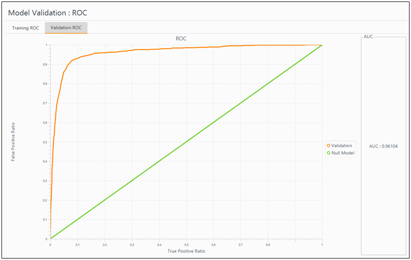
Figure 5: DMWay output for a logistic regression model
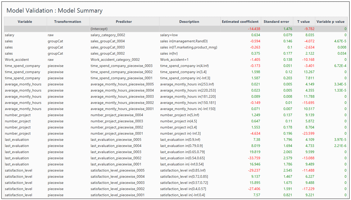
Figure 6: DMWay output for significant variables
The model made by DMWay outperform the logistic regression in R. Perhaps more efforts in feature selection would have yield better results in R. But faster and better predictive models is the whole point of using DMWay. Ronen Meiri – Ph.D., Founder, and CTO of DMWay, explains that “DMWay automated solution is powered by a sophisticated analytic engine that mimics all the steps taken by experienced data scientists during the analytic process.” This may take weeks or months sometimes. “DMWay is led by leading data science experts”, says Meiri, “and encompasses many years of researching automation and simulating the work of a data scientist. While building predictive analytics models in the world of big data is time-consuming, costly, and risky, DMWay offers everyone the ability to build better predictive models in a matter of hours.”
The next step: Deployment
According to the data mining process known as CRISP-DM, the next step after modeling and evaluation is deployment, namely putting the model in real use. While deploying a model generated in R involves excessive work, mainly to translate it to other programming languages used in the organization, DMWay offers an innovative solution: At the end of the model generation process, it can generate the code for deployment, in three programming languages: R, SQL, and Java. This code is ready for export to the organization’s database.
Does it mean that our fiction organization should now hurry to predict which of its best employees is the next to leave? Although it is technically possible, it is not ethically recommended. The only reason that I mention deployment in this context, is for mentioning this additional strength of DMWay. There are many other business outcomes related to employees that it would be wise to predict and deploy, however, in my opinion, pointing the next employee who is at “flight risk” in a certain moment, is not one of them.
The ethical issue of predicting employee attrition has been long discussed, e.g., in the context of civil rights. I would use this specific model to understand employee attrition, in order to reduce it, or to test the impact of some organizational interventions, though. I think that when pointing to an employee that is not 100% intent to leave, there is a chance for different results, not all in favor of that employee. Furthermore, we should all remember that models will be always models, they can’t encompass the whole reality. The British statistician George E. P. Box said it most appropriately: “Essentially, all models are wrong, but some are useful”.
And the winner is…?
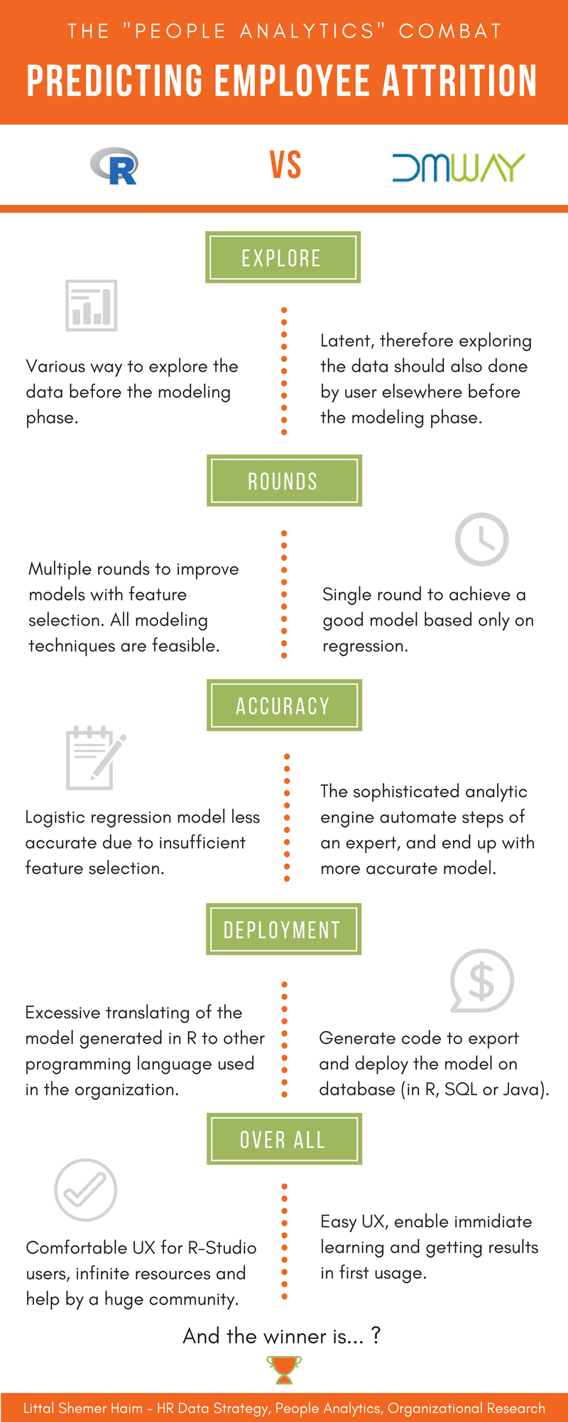
To wrap up our test, let’s come back to the story of David and Goliath. As you probably recall, David goes into battle with only a sling – a simple and common tool among shepherds. He walks right up to Goliath and kills him with a single shot to the head. DMWay’s sling is not simple nor common. But for contemporary business analysts, data scientists, domain experts, and also executives, it turns out that it is effective to defeat the giant R, in terms of time-consuming, model accuracy, and deployment. The whole process of this battle is summarized in the following infographics.
Yet, to be honest, our fiction battle ends differently. In contrast to the biblical story, our giant is not defeated but rather lives happily ever after, since he is “open”, i.e., letting others to use his power. In fact, like much contemporary software, DMWay relies on R in the backstage.
So which tool would you pick for predicting employee attrition?
I’ll appreciate sharing your thoughts in a comment.
An overview of future role of HR leaders in improving business performance by informed decisions about people based on data. People Analytics transforming HR; The Role of People Analytics Leader; Case Studies and Simulations; Emerging trends of HR tech.





5 thoughts on “Predicting Employee Attrition: R vs DMWay”
מעניין מאד. סקירה מקצועית ורלוונטית לנו, אנשי משאבי אנוש
“The data science language R is a convenient tool for performing HR churn prediction analysis. A lightweight data science accelerator that demonstrates the process of predicting employee attrition is shared…” here: http://blog.revolutionanalytics.com/2017/03/employee-retention.html
Here is another demo of churn prediction (An example in the domain of customer relationship management, which can be easily converted to the field of the workforce), by mljar.com service and its R API. With just a few lines of code, it enables very good results. This tool frees the user from thinking about model selection. It uses various machine learning algorithms and compares their performance.
If you’re interested in using Machine Learning for employee turnover prediction and explanation, and R applications in business, check out this 30 minute presentation from EARL Boston 2017: http://www.business-science.io/presentations/2017/11/06/earl-boston-2017.html (Page includes link to code).
Pingback: Having Trouble with Employee Turnover? People Analytics Can Help Your HR – and Business
Comments are closed.